Waves 1
Table of Contents
- 1. Functional form of wave
- 2. Energy stored in a travelling transverse wave
- 3. Average Power of superposition of two sinusoidal waves (antiparallel)
- 4. Energy per unit length of superposed sinusoidal wave (anti-parallel)
- 5. Power of superposition of two sinusoidal waves (parallel)
- 6. Energy per unit length of superposed sinusoidal wave (parallel)
- 7. Reflection and Transmission of waves
- 8. Superposition and Interference of transverse waves
- 9. Resonance (Standing waves in string)
- 10. Alternate way of looking resonance
1. Functional form of wave
For right travelling wave: \[ y = f\left( t-\frac{x}{v} \right) \qquad \text{or} \qquad y = f(x-vt ) \]
For left travelling wave: \[ y = f\left( t+\frac{x}{v} \right) \qquad \text{or} \qquad y = f(x+vt ) \] Here, wave velocity is \( v \).
1.1. Restrictions on \( y = f(x-vt) \)to represent a “physical” wave
- \( y \) must be continous.(otherwise string will break)
- \( y \) must be differentiable.(sudden slope change would cause infinite acceleration)
- \( y \) must be bounded.(Any material particle cannot have infinite displacement)
\( y = e^{- (4x-3t)^2} \) represents equation of a physical wave since it is bounded whereas \( y = e^{(x-4t)} \) does not because it is not bounded.
1.2. Shifting of wave equation
If for a certain location(\( x_0 \)), the disturbance is given by \( y = f(t) \), then at a general location \( x \) it will be given by \[ y = f\left( t - \frac{x-x_0}{v} \right) \] Similarly, if at a general time(\( t_0 \) ), the equation of wave is given by \( y = f(x) \) , then at a general time it will be given by \[ y = f (x - v(t-t_0)) \] These two shifting properties are used in transformation of waves such as \( \pi \) shifts.
2. Energy stored in a travelling transverse wave
Let: \[ G = \left( \frac{\partial y}{\partial t} \right)^2 + v^2 \left( \frac{\partial y}{\partial x} \right)^2 \] Amount of energy stored in a small segment of a travelling transverse wave: \[ \mathrm{d}E = \frac{1}{2}\mu \ G \ \mathrm{d}x \] Energy per unit length: \[ \frac{\mathrm{d} E}{\mathrm{d} x} = \frac{1}{2} \mu G \]
Note: The energy is equally divided between kinetic and potential energy.
The average value of each term inside the brackets is \( 1 /2 \) .
For a sinusoidal wave \[ \left< G \right> = A^2 \omega^2 \]
\[ \left< E \right> = \frac{1}{2} \mu A^2 \omega^2\]
2.1. Power generated
In general: \[ P = -T\left( \frac{\partial y}{\partial x} \right) \frac{\partial y}{\partial t} \] \[ = -T v \left( \frac{\partial y }{\partial x} \right)^2 \]
For progressive waves: \[ = \frac{1}{2} \mu\ v \ G \]
Average power generated: \[ \left< P \right> = \frac{1}{2} \mu v A^2 \omega^2 \]
2.2. Intensity
\[ I = \frac{P}{S} = - \frac{T}{S} \left( \frac{\partial y}{\partial x} \right) \frac{\partial y}{\partial t} \] For progressive wave: \[ = \frac{1}{2} \frac{\mu v G}{S} \] \[ = \frac{1}{2} \rho vG \] Average Intensity: Same as average power, \[ \left< I \right> = \frac{1}{2} \rho v^2 A^2 \omega^2 \]
3. Average Power of superposition of two sinusoidal waves (antiparallel)
Let the wave function of a wave travelling in a string be: \[ y = A \sin(kx - \omega t + \phi_1) + B\sin (kx + \omega t + \phi_2) \] Then \[ \left< P \right> = \frac{Tk \omega}{2} \left[ A^2 - B^2 \right] \] Power of opposite travelling waves have opposite signs.
Instantaneous power: \[ P = P_1 + P_2 \] \[ \left< P \right> = \left< P_1 \right> + \left< P_2 \right> \] Thus power of superposition of two oppositely directed sinusoidal waves is simple superposition of powers of individual compound.
4. Energy per unit length of superposed sinusoidal wave (anti-parallel)
\[ e_{\ell} = \frac{1}{2} \mu \left[ \left( \frac{\partial y}{\partial t} \right)^2 + v^2 \left( \frac{\partial y}{\partial x} \right)^2 \right] \] \[ \implies e_{\ell} = e_{\ell_1} + e_{\ell_2} \]
5. Power of superposition of two sinusoidal waves (parallel)
Consider a wave: \[ y = y_1 + y_2 = A \sin(kx - \omega t + \phi_1)+ B \sin (kx - \omega t + \phi_2) \]
The power in this case is given by: \[ P = P_1 + P_2 + 2\sqrt{P_1P_2} \] (Note the extra \( 2\sqrt{P_1P_2} \) ) term.
Average power: \[ \left< P \right> = \left< P_1 \right> + \left< P_2 \right> + 2\sqrt{\left< P_1 \right> \left< P_2 \right>} \cos \left( \Delta \phi \right) \]
Average Intensity: \[ I = I_1 + I_2 + 2\sqrt{I_1 I_2} \cos \left( \Delta \phi \right) \]
6. Energy per unit length of superposed sinusoidal wave (parallel)
\[ e_{\ell} = e_{\ell_1} + e_{\ell_2} + 2 \sqrt{e_{\ell_1} e_{\ell_2}} \] Average power: \[ \left< e_{\ell} \right> = \left< e_{\ell_1} \right> + \left< e_{\ell_2} \right> + 2 \sqrt{\left< e_{\ell_1} \right> \left< e_{\ell_2} \right>} \cos \left( \Delta \phi \right) \]
7. Reflection and Transmission of waves
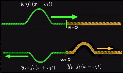
At \( x= 0 \) : \[ y_i + y_r = y_t \] (From unbreakability of string) Differentiating with respect to \( x \) , \[ y_i' + y_r' = y_t' \]
At boundary: \[ \dot{y}_i + \dot{y}_r = \dot{y}_t \] Also, \[ y_i' = -\frac{1}{v_1} \dot{y}_i \] similarly for reflected and transmitted wave….
Substituting, \[ - \frac{1}{v_1} \dot{y}_i + \frac{1}{v_1} \dot{y}_r= - \frac{1}{v_2} \dot{y}_t \] Solving the two differential equations,
\[ \dot{y}_t = \frac{2v_2}{v_1 + v_2} \dot{y}_i \]
\[ \dot{y}_r = \frac{v_2 - v_1}{v_2 + v_1} \dot{y}_i \]
\[ \implies y_t = \frac{2v_2}{v_1 + v_2}y_i \qquad y_r = \frac{v_2 - v_1}{v_1 + v_2} y_i \]
Our derivation is independent of location of reflecting boundary.
7.1. Steps for finding reflected and transmitted waves
Suppose we have reflecting boundary at \( x = a \) and our incident wave is \( y_i = f(x-v_1t) \), then we follow these steps:
- Evaluate incident disturbance at \( x = a \) , \( y_i = f (a-v_1t) \)
- Calculate transmitted disturbance as \(\displaystyle y_t = \frac{2v_2}{v_1 + v_2} f(a-v_1t) \)
- Calculate transmitted wave by applying a future shift of \( \displaystyle \left( \frac{x-a}{v_2} \right) \) to \( y_t \) at the boundary i.e. \[ y_t = \frac{2v_2}{v_1 + v_2} \times f \left( a - v_1 \left[ t- \frac{(x-a)}{v_2} \right] \right) \]
- Calculate reflected disturbance at the boundary as \( \displaystyle y_r = \frac{v_2 - v_1}{v_1 + v_2} \times f (a-v_1t) \)
- Calculate reflected wave by future shifting by \( \displaystyle \left( \frac{a-x}{v_1} \right) \) i.e. \[ y_r = \left( \frac{v_2 -v_1}{v_1 + v_2} \right) \times f \left( a - v_1 \left[ t- \frac{(a-x)}{v_1} \right] \right) \]
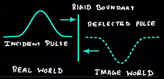
7.2. Reflection from a rigid boundary
At fixed boundary, there can be no displacement, thus \[ y_r = - y_i \] \[ \implies y_r = \left( \frac{v_2 - v_1}{v_1 + v_2} \right) y_i = - y_i \] i.e. the wave just inverts. It can be modelled as an superposition with an inverted imaginary wave coming from boundary.
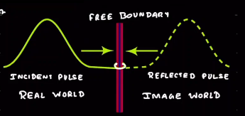
7.3. Reflection from a free boundary
A free boundary is modelled as end of a string attached to a massless ring free to slide in a frictionless rod. Since the ring is massless therefore it can’t have any vertical component of tension acting on it. Therefore the slope of the string at this boundary must always be zero. \[ \dot{y}_i = \dot{y}_r \] \[ \implies y_i = y_r \] \[ y_r = \left( \frac{v_2 - v_1}{v_1 + v_2} \right) y_i \] Since, \( v_2 \to \infty \) , \[ y_r = y_i \] It can be modelled as an superposition with an imaginary wave coming from boundary.
7.4. Energy transmission and reflection across a boundary
Incident power: \( \mu_1 v_1 \dot{y}^2_i \) Reflected power: \( \mu_1 v_1 \dot{y}^2_r \) Thus, reflected fraction: \[ \eta = \left( \frac{\dot{y}_r}{\dot{y}_i} \right)^2 \] \[ \implies \eta = \left( \frac{v_2 - v_1}{v_1 + v_2} \right)^2 \] Transmitted fraction: \[ \eta_t = 1 - \left( \frac{v_2 - v_1}{v_1 + v_2} \right)^2 \] \[ = \frac{4v_1 v_2 }{(v_1 + v_2)^2} \]
The reflected and transmitted fraction are same for \( \displaystyle \frac{v_2}{v_1} = \lambda \) or \( \displaystyle \frac{v_1}{v_2} = \lambda \) : \[ \eta_r = \left( \frac{v_2 - v_1}{v_1 + v_2} \right)^2 = \left( \frac{\frac{v_2}{v_1} - 1}{\frac{v_2}{v_1} + 1} \right)^2 = \left( \frac{\frac{v_1}{v_2} - 1}{\frac{v_1}{v_2} + 1}\right)^2 \]
Since, \( \displaystyle P_i = \frac{1}{2} \mu v A_i^2 \omega^2 \) and \( \displaystyle P_r = \frac{1}{2}\mu v A_r^2 \omega^2 \) , we get: \[ A_r = \left( \frac{v_2 - v_1}{v_1 + v_2} \right)A_i \qquad \text{and} \qquad A_t = \left( \frac{2v_2}{v_1 + v_2} \right) A_i \]
8. Superposition and Interference of transverse waves
The wave equation is governed by the differential equation: \[ \frac{\partial^2 y}{\partial t^2} = v^2 \frac{\partial^2 y}{\partial x^2} \] If there are two solutions: \[ f(x-vt) \qquad \text{and} \qquad g(x+vt) \] Then, the differential equation is also satisfied by \[ y = f(x-vt) \pm g(x+vt) \] i.e. waves follow superposition theorem.
Note: For obeying the superposition principle, mechanical waves must have small amplitudes. If amplitude is too large, medium is distorted past the limit where the restoring forces are linearly proportional to the deformations.
8.1. Stationary Waves
Whenever two waves of same amplitude travelling in opposite direction superpose, we get what are known as stationary waves.
Let there be two waves: \[ y_1 = A\sin(kx - \omega t) \] \[ y_2 = A \sin (kx + \omega t) \] \[ y = y_1 + y_2 = 2A \sin (kx) \cos (\omega t) \]
8.1.1. Position of Nodes and Antinodes
For nodes: \[ \sin (kx) = 0 \] \[ \implies kx = n\pi \]
\[ \implies x = \frac{n}{2}\lambda \]
For antinodes: \[ \sin(kx) = \pm1 \] \[ \implies kx = (2n+1) \frac{\pi}{2} \]
\[ \implies x = \frac{2n+1}{4} \lambda \]
The nearest distance between two nodes/antinodes is \( \lambda /2 \) and between one node and antinode is \( \lambda /4 \) .
8.1.2. Power transmission in stationary waves
Recalling from power equation: \[ P = -T \left( \frac{\partial y}{\partial t} \right) \frac{\partial y}{\partial x} \] At antinode, slope is zero and at node, particle velocity is zero, hence there is no power transmission. Thus energy is trapped between node and antinode.
At nodes, entire energy is stored as potential energy and at antinodes, entire energy is stored as kinetic energy.
For oppositely travelling wave, we can use the superposition principle: \[ e_{\ell} = e_{\ell_1} + e_{\ell_2} \]
Note: \( e_{\ell} \) at \( \lambda /4 \) is independent of time and is equal to \( \mu A^2 \omega^2 \).
8.1.3. Energy stored in a standing wave
\[ \mathrm{d}m = \mu \ \mathrm{d}x \] The energy of the particle at \( \mathrm{d}x \) is \[ \mathrm{d}E = \frac{1}{2}\mathrm{d}m \ v^2 \] Substituting the value of \( \mathrm{d}m \) and \( v \) from the equations, we get \[ \mathrm{d}E = \frac{1}{2} \mu \ \mathrm{d}x (2A\omega \sin kx) ^2 \] \[ = \frac{1}{2} \mu \ \mathrm{d}x \left( 4A^2 \omega^2 \sin^2 kx \right) \] The total energy can be determined by integrating between \( 0 \) and \( \lambda /2 \) :
\begin{align*} E_T &= 2A^2 \omega^2 \mu \int_0^{\lambda /2} \sin^2 kx \ \mathrm{d}x \\ &= 2A^2 \omega^2 \mu \int_0^{\lambda /2} \left( \frac{1-\cos(2kx)}{2} \right) \mathrm{d}x \\ &= A^2 \omega^2 \mu \left[ \int_0^{\lambda /2} \mathrm{d}x - \int_0^{\lambda /2} \cos (2kx) \mathrm{d}x \right] \\ &= A^2 \omega^2 \mu \left[ \frac{\lambda}{2} - \left[ \frac{\sin 2kx}{2k} \right]_{0}^{\lambda /2} \right] \\ &= A^2 \omega^2 \mu \frac{\lambda}{2}\\ &= A^2 \omega^2 \mu L \end{align*}Therefore, the total energy of the loop in a standing wave is \[ E_T = A^2 \omega^2 \mu L \] Here, \( L \) is the length of loop.
9. Resonance (Standing waves in string)
9.1. String fixed at both ends
9.1.1. First harmonic (Fundamental)
\[ L= \frac{\lambda}{2} \] \[ \nu = \frac{v}{2L} \]
The least frequency for which resonance occurs is called fundamental and all it’s multiples are called harmonics.
\( N^{th} \) harmonic: \[ \nu = \frac{nv}{2L} \]
Overtone number: If all natural frequencies of a system are arranged in ascending order and numbered sequentially beginning with zero, then number corresponding to each frequency is called overtone number.
9.2. Strings fixed at one end and free at one end
9.2.1. Fundamental frequency
\[ L = \frac{\lambda}{4} \] \[ \nu = \frac{v}{4L} \]
9.2.2. First overtone (third harmonic)
\[ \nu = \frac{3v}{4L} \] \( N^{th} \) harmonic: \[ \nu = (2n+1) \frac{v}{2L} \]
| \( n \): | Overtone number |
| \( (2n+1) \) : | Harmonic number |
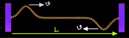
10. Alternate way of looking resonance
Suppose we generated a pulse (in a string fixed at both ends), the pulse will return to the same point after a time \( 2L /v \). If we generate another pulse, the amplitude of the pulse increases.
Same argument goes for any fractional time of \( 2L /v \) , we are just increasing the number of pulses, but the logic gets the same.
Note: This argument can be used for finding natural frequencies in string having variable mass density.